I recently encountered the problem where I was trying to add a filter on the top row but Excel kept putting it on the second row.
Here’s a picture of this annoying problem:
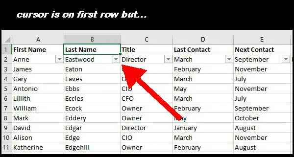
Although I have placed the cursor on the first row and the B1 cell is highlighted, Excel insists on putting the filter on the second row.
I finally found an old solution in a forum post dated back in 2007. Microsoft has changed the interface a lot since then, so I had to “translate” the information to get it to work.
I’ll give you the quick solution first and then go into the reasons behind the problem.
Table of Contents
Quick Fix To Getting The Filter On The First Row
Take these steps to fix the issue.
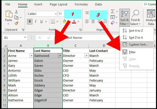
- Click on any column header to highlight the entire column
- Expand the Sort & Filter menu
- Click the Filter menu item (this clears the current filter)
- Click the filter item again (this adds the new filter in the correct place)
I’ve highlighted steps 1 and 3 in the picture below.
Reason For The Problem
Feel free to bail and keep working with Excel if you don’t want to know why the problem happened in the first place. But if you’re curious, read on.
The problem is that Excel retained in its memory a previous range or filter that you had set that didn’t include the first row. So, it is “helpfully” predicting that you want to filter the same range.
This doesn’t necessarily mean a range you applied a few minutes ago. When I encountered the problem, it was when I opened an Excel spreadsheet that I had worked with and closed the previous day.
The solution of highlighting a full column is that it tells Excel that you want to use a new range that doesn’t start on the second row!
What Doesn’t Work
Highlighting a full column was the only method that I could get to work.
I also tried freezing the top row. Well, it was already frozen, so I undid the setting and reapplied it. This didn’t fix the issue.
I even inserted a new row to push the content down by one row. But Excel continued to be frustratingly “helpful” and simply added the filter down on the third row.
One thing I didn’t try was copying the content into a new worksheet. I assume that would have worked simply because by highlighting the entire content, a new range would now be set.
But this set of steps would be more clicks and work than simply highlighting a single column.
Other Annoying Excel Problems
Isn’t it great when you look for answers to a “new” Excel problem and find that one of the earliest complaints about it is back in 2005? Microsoft is nothing if not consistent!
If you use a shape to make a nice-looking button for your macros, be sure to test the worksheet repeatedly. You may find that your button simply…goes away. If that happens, check out my article on how to fix an Excel shape that disappears.